Imaging: Synchronisation

The two-photon miniscopes make use of multiple independent time series data streams - imaging, tracking, running wheel etc. Synchronisation is the process of converging all of those separate time-series data, which may be derived from independent, unique, clocks that do not fully agree with one another, into a single temporal frame of reference.

The outcome of that synchronisation stage should more properly be called time information, but throughout the Imaging pipeline is often also called synchronisation data.

Three methods are currently in use within the Moser group:

• Wavesurfer with a National Instruments GPIO card

• Femtonics Mesc synchronisation

• ScanImage Presynchronisation

Each of these implementation is then inserted into a very generalised schema, which maps the time data from each time series into a single temporal frame of reference. This generalised approach has both benefits and drawbacks: the primary benefit is that it can be extended to new types of data - and new hardware - very easily. The primary drawback is that it adds complexity and overhead to common operations, and that the users need to be aware of that complexity.

Synchronisation data is stored in the Sync table and its sub-tables.

Each Session is generated by a System (Systems and Scopes), which is tracked in the SystemConfig table. Each entry in the SystemConfig table has a list of the types of synchronisation data (and how to interpret it) that might be generated in the table SystemConfig.Sync.:

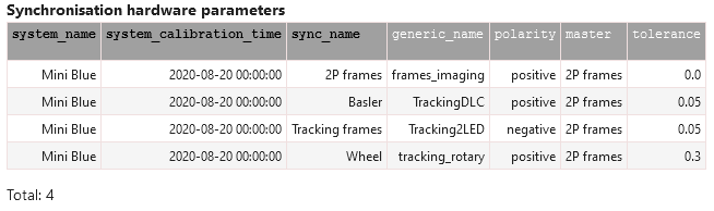
SystemConfig.Sync & {"system_name":"Mini Blue", "system_calibration_time":"2020-08-20 00:00:00"}

When a new Recording is ingested, the synchronisation data is inserted into the Sync table and its part tables. Each Recording has one (or more) entries in the Sync table, corresponding to a single time series, from a single instrument, with each time series being identified by a sync_name.

The actual timestamps themselves are stored in the column sync_data of the Sync table. The values are stored in whatever unit the underlying synchronisation system stores, which may be converted into seconds via the conversion factor in sample_rate.

• Wavesurfer synchronisation stores data in samples

• ScanImage pre-synchronisation stores values in seconds (sample_rate = 1)

Sync Names and Generic Names

The SystemConfig.Sync entries have two related attributes:

• sync_name

• generic_name

The distinction here is between what the raw data files call a synchronisation stream (sync_name) vs a common name that the imaging pipeline logic searches for (generic_name).

• frames_imaging : timestamps for two-photon imaging frames. For Multiplane data, this corresponds to the start time of scanning a volume. Consequently, there should be the same number of data points in frames_imaging as there are data points for the fluorescence value of a single cell.

• tracking_rotary : timestamps of 1-dimensional, wheel-encoder data

• Tracking2LED : timestamps of video frames of open-field tracking, where the subject is identified by a pair of head-mounted LEDs

• TrackingDLC : timestamps of video frames intended to be analysed with DLC (see Imaging: DLC).

In most cases, users should not need to extract data from the Sync tables directly: timestamp information is inserted into the more common tables (Tracking.Linear, Tracking.OpenField, SignalTracking).

When the Synchronisation table is populated, it will look up what SystemCOnfig was used to record the Recording (via Session.SystemConfig), and then look up the appropriate names for each kind of sync stream (via SystemConfig.Sync). This is demonstrated in the example below. A utility function is also provided for the same purpose (utils.get_sync)

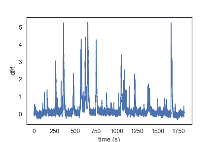
# Use an arbitrary key to the `Cell.Traces` table
key = {"recording_name":"d6ba671faad74695", "cell_id":3, "channel":"primary"}
df_f = (Cell.Traces & key).fetch1("df_f")

# Identify what system was in use
system = (Recording * Session.SystemConfig & key).fetch1()

# Identify what sync name we should be looking for
generic_name = "frames_imaging" # cell.Traces data -> it's from the 2p data
sync_name = (SystemConfig.Sync & system & {"generic_name":generic_name}).fetch1("sync_name")

# Get the sync data and sampling rate, and convert from samples to seconds
sync_data_samples, fs = (Sync & key & {"sync_name":sync_name}).fetch1("sync_data", "sample_rate")
sync_data_s = sync_data_samples / fs

# Plot the resulting data
fig, ax = plt.subplots()
ax.plot(sync_data_s, df_f)
ax.set_ylabel("df/f")
ax.set_xlabel("time (s)")

Wavesurfer sync

Multiple independent instruments acquire data at their own sampling frequency, whatever that is. Each time a sample is taken, that instrument outputs a TTL pulse. A single GPIO device recieves those signals, with a single channel dedicated to each device. The timestamps (and sampling frequencies) for each of those devices is determined by the GPIO device’s own clock, thus providing a single temporal frame of reference (customarily called a “master clock”.

At present, this uses Wavesurfer software running on a computer with a National Instruments GPIO card, but the method is generalisable to any GPIO device and associated software to interface with it.

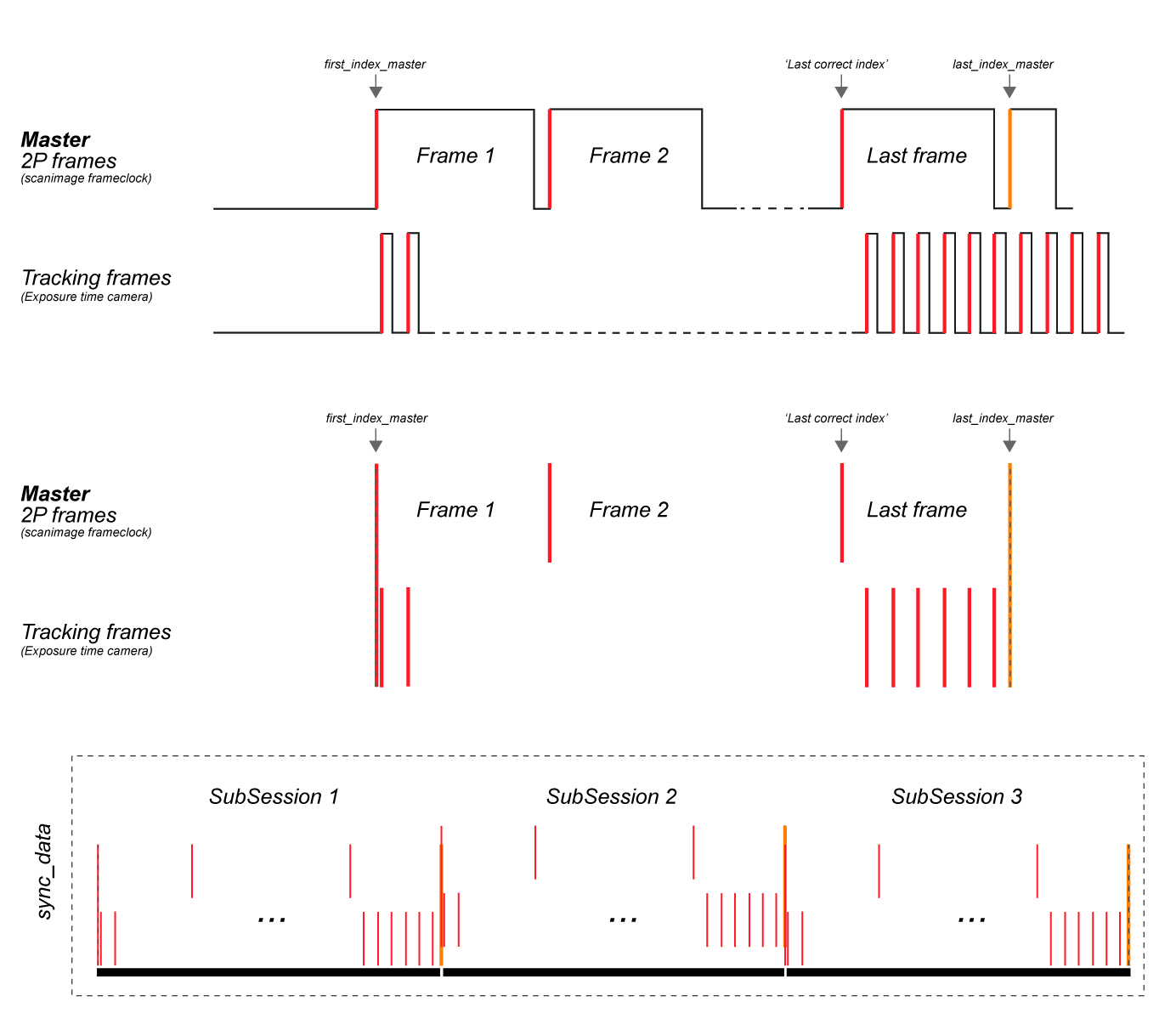
Below is an example of the raw recording of 3 sync streams (digital inputs) via wavesurfer. After an initial delay, the acquisition is triggered and the scanning starts (2P frames, master). At the same time the camera for tracking of 2 LEDs is triggered and every exposure is registered (Tracking frames). The (Wheel) stream records serial events that are sent from a microcontroller that is registering data from a rotary encoder attached to a running wheel (irregular since script wasn’t running).

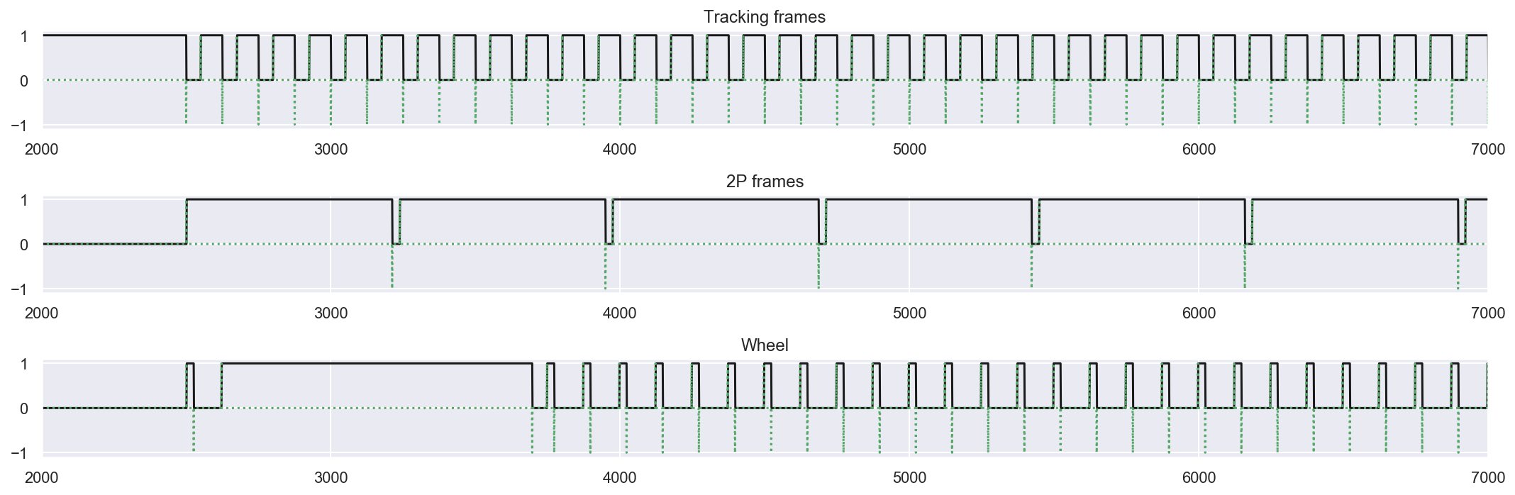
Events are extracted according to the polarity of the digital signal - i.e. rising or falling edge - and shown on the image below as red bars. A last_index_master is inferred (since not actually recorded) and the other sync streams are cut accordingly. To concatenate multiple (sub-)sessions, sync streams are zeroed on master (first_index_master) and every subsequent sync stream is concatenated to the previous one adding 1 to last_index_master.

Wavesurfer stores its data in an hdf5 container. A reader for these containers is provided under /helpers/mini2p_wavesurfer.py.

Scanimage sync

The OpenMiniscope system implements one particular special case of the more general synchronisation scheme outlined above. Data can be pre-synchronised with the ScanImage software.

In the case of “pre-synchronisation”, every instrument that is used is triggered by a signal sent from the “master” device, which is typically the device that acquires data directly from the two-photon imaging system. Each time that the laser scanner begins a new scan, a TTL signal will be sent to the subject tracking camera, causing it to record a tracking frame at the same time (or with a constant, known, offset delay).

In the case of multi-plane imaging, a TTL signal will be sent at the start of each plane. Therefore, for a cell present in one plane out of N imaged planes, the tracking data will have N times more data points than the cell has fluoresence data points, and it is necessary to select the appropriate data points to be matched. For example, if the two-photon microscope is scanning an entire volume every 100 ms (10Hz), and the volume contains 2 planes, then the tracking camera will record every 50 ms (20Hz).

For instruments where the acquisition rate of the two-photon imaging frames is too slow, a much higher rate of data may be transmitted to the “spare” imaging channels, with the data being saved as an array stored as another Tif. This method does not directly provide higher temporal resolution, since the timestamp data is only recorded per-Tif, and not per-Tif-pixel: a higher temporal resolution may be approximately inferred

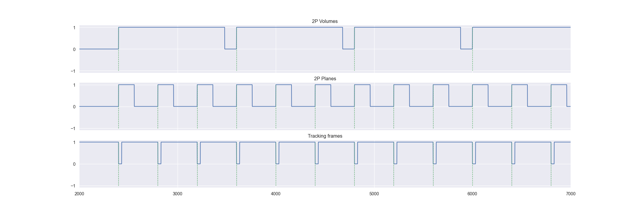
In the case of pre-synchronised ScanImage data, a Tracking frame is generated every time a new plane acquisition starts.

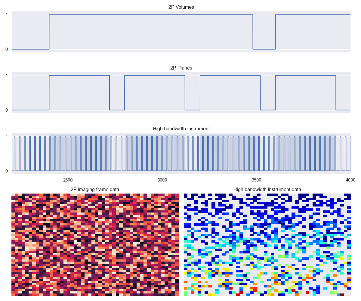
Where 1:1 sampling frequency is not adequate, an external instrument running on its own independent clock can feed data into one of the spare imaging channels, with data saved as an additional tif layer per plane.

Note that this approach has some drawbacks: data is streamed into the tif in parallel with the timing of the laser scanner, which may result either in un-recorded data (instrument faster than laser scanner) or empty pixels (instrument slower than laser scanner). Any non-linearity in the per-pixel timing owing to the non-linear behaviour of the laser scanner must be accounted for when inferring the per-pixel timing.

Femtonics Sync

For the femtonics setup (.mesc files), the internal oscilloscope function is used to record events in sync with acquisition (see /helpers/femto_mesc.py).