Imaging: The basics¶

After completing the instructions under Getting Started with Datajoint (Python), these next steps will show you how to add data to the pipeline and evaluate some of its outputs (which cells does it identify and what are their functional properties?).

Workflows¶

Primary workflows¶

Most interactions with the imaging pipeline will be either:

Adding data to the pipeline after recording. Mostly done via the Imaging: Web GUI
Evaluating cells identified by Suite2p or other algorithm. Evaluate the cells Suite2p identified in your data
Fetching data from the pipeline for analysis. See Fetching for how this works, and the Imaging: Helper notebooks for examples of how to work with your data

Less common processes¶

A few less common activities to be aware of:

If a new system or scope is developed and used, new entries should be added to the pipeline to represent these physical entities
- A scope is the microscope objective - it (partially) controls factors such as field of view, and the unwarping routine used to correct for the distortion of the field of view
- A system is pretty much everything else in the room except the arena and the subject. It keeps track of the most recent calibration data, hardware configuration, etc.
New subject implants can be recorded in the Implant table. There is currently no user interface other than code to work with this table
Parameter sets. Most analysis steps in the pipeline offer the ability to choose different parameters. An interface for this system is under development.

Add imaging data to the pipeline¶

The easiest way to do this is via the web gui, (Imaging: Web GUI), although it may also be done via Python or Matlab code if you prefer.

Evaluate the cells Suite2p identified in your data¶

Suite2p is an imaging processing pipeline for registering images and detecting cells and spikes. It is written by Carsen Stringer and Marius Pachitariu. To sort through the cells it has identified in your data, discarding artefacts etc that shouldn’t be added to the pipeline, you first need to install Suite2p locally so you can use the Suite2p GUI.

Install Suite2p¶

If you are familiar with git, you can follow the installation instructions in the suite2p documentation. If not, then these steps might be more intuitive:

Download GitHub Desktop (this is a useful program for interfacing with GitHub, learn more).
Within GitHub Desktop, go to File -> Clone repository…
Select the URL tab, add the link to the suite2p repository (https://github.com/MouseLand/suite2p) and select a location in which to save it (e.g. locally on your computer).
Click Clone
Open an Anaconda Prompt and change the directory to where the environment.yml file in the suite2p repository folder is, e.g.:
- (base) $ cd C:\User\me\Code\suite2p
Create a separate suite2p environment based on the environment.yml file
- (base) $ conda env create -f environment.yml
Activate the new suite2p environment
- (base) $ conda activate suite2p
Install suite2p
- (suite2p) $ pip install suite2p

Identify cells to keep¶

With suite2p installed, you can open the GUI via the Anaconda Prompt after activating the suite2p environment:

(base) $ conda activate suite2p
(suite2p) $ suite2p

You can find the documentation for how to use the Suite2p GUI, but here are a few basic steps to get your started:

Locate the stat.npy file that suite2p generated when it ran through your analysis (the path may look something like this:
- N:\Ragnhild\Mouse 000\YearMonthDate\MUnit_0\suite2p\plane0 or
- N:\Ragnhild\Mouse 000\YearMonthDate\combined_xxx\mini2p_GC6m1\plane0.
- Details on the folder logic can be found here.
Drag and drop the stat.npy file into the suite2p GUI or open it via File -> Load processed data in the GUI.
Use the buttons along the top of the GUI to determine your view (the buttons named cells - both - not cells): click both to see the ROIs that suite2p has picked out as cells on the left, and ROIs that it has discarded on the right.
Left click any ROI to see its associated trace at the bottom of the GUI.
Right click any ROI to move it from one category to another (e.g. right clicking on an ROI in the cells panel will move it to the not cells panel). NOTE: changes are saved automatically to the stat.npy file.
When you have finished, i.e. you have all the ROIs you want to keep in the cells window, go back to Suite2p -> Finished Suite2p Jobs in the web GUI
Click the Add button by your session only once to tell the pipeline to incorporate the ROIs you have selected. The pipeline will now calculate ratemaps etc for every ROI - this will take time.
While the pipeline is working hard adding your cells, you can take a well deserved break and check the progress by, for example, following these steps:
- Identify the Recording hash of your session by filtering under Recordings in the imaging web GUI.
- Execute these commands within a jupyter notebook, using your session hash between the double quotes:

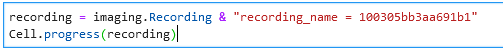
NOTE: if you decide to re-sort the ROIs, you can follow the exact same steps, including using the Add button to notify the pipeline of the change, but only click Add after the progress indicator has reached 100%. If the Add button is no longer there (because it has been more that 14 days), you can re-add the Basefolder (What happens if I don’t like this or that cell from the suite2p output?).

If suite2p hasn’t done a good job of identifying cells, it may be worth creating your own options file with settings tuned specifically to your data (see below).

Create a new suite2p options file for your data¶

For inspiration, check out the current option files being used, and their contents, in the imaging web GUI under Suite2p -> Manage Suite2P Options.

To create your own:

Open the suite2p GUI and go to File -> Run suite2p
Modify the options to you want to change.
Click ‘Save ops to file’ to save a new options file.
Test these new options on your data (without involving the pipeline):
- Click Add directory to data_path to choose the folder that contains your raw data.
- If you already have a suite2p folder in that location, move it to another folder if you want to keep it, or delete it.
- Click RUN SUITE2P (the panel below will show the analysis progress and let you know when it’s finished).
- The analysis output will automatically load into the suite2p GUI where you can evaluate it.
When you are happy with your modified options, make this new options file available in the imaging web GUI by uploading it under Imaging -> Suite2p -> Add Suite2p Options
Notify the pipeline to use the new ROIs you’ve obtained on your data (What happens if I don’t like this or that cell from the suite2p output?)

Check out the functional properties of your cells¶

Your data has been ingested and cells identified, so now it’s finally time to check if they have any interesting properties! Datajoint automatically calculates all sorts of things for you, including each cell’s ratemap and grid score, and a nice way to look at them is via the Imaging: Recording Viewer made by Horst Obenhaus. The documentation that link leads to also tells you which tables the GUI is collecting the data from, which is a helpful reference for when you start fetching and plotting data from the pipeline on your own.

You’re now ready to delve deeper into the pipeline and start analysing all your cool data. May all your analysis dreams come true! (but if they don’t, the Support channel on Teams is here to help)