Imaging: Recording Viewer

Recording Viewer is a desktop application for screening individual recordings in the Imaging pipeline.

Installation

Prior to 2021-05-05, the recording viewer was installed separately. Subsequent to this date, it is recommended to install the viewer simultaneously with general set up for working with the imaging pipeline.

To install separately, or in another environment, or to update to the latest version, run the following command:

(your_environment) $ pip install git+https://github.com/kavli-ntnu/dj-imaging-user.git -U

Running

Running the gui relies upon you already having configured your Datajoint credentials and saved them with dj.config.save_global(), see Getting Started.

To start the viewer GUI, run the following command in your terminal:

(imaging) $ recording_viewer

Overview

Once started, you can copy/paste a recording_name hash into the text field on the top left and press enter (next to Recording:). This will load and display this recording from the database. recording_name hash refers to the recording_name attribute of every recording in datajoint.


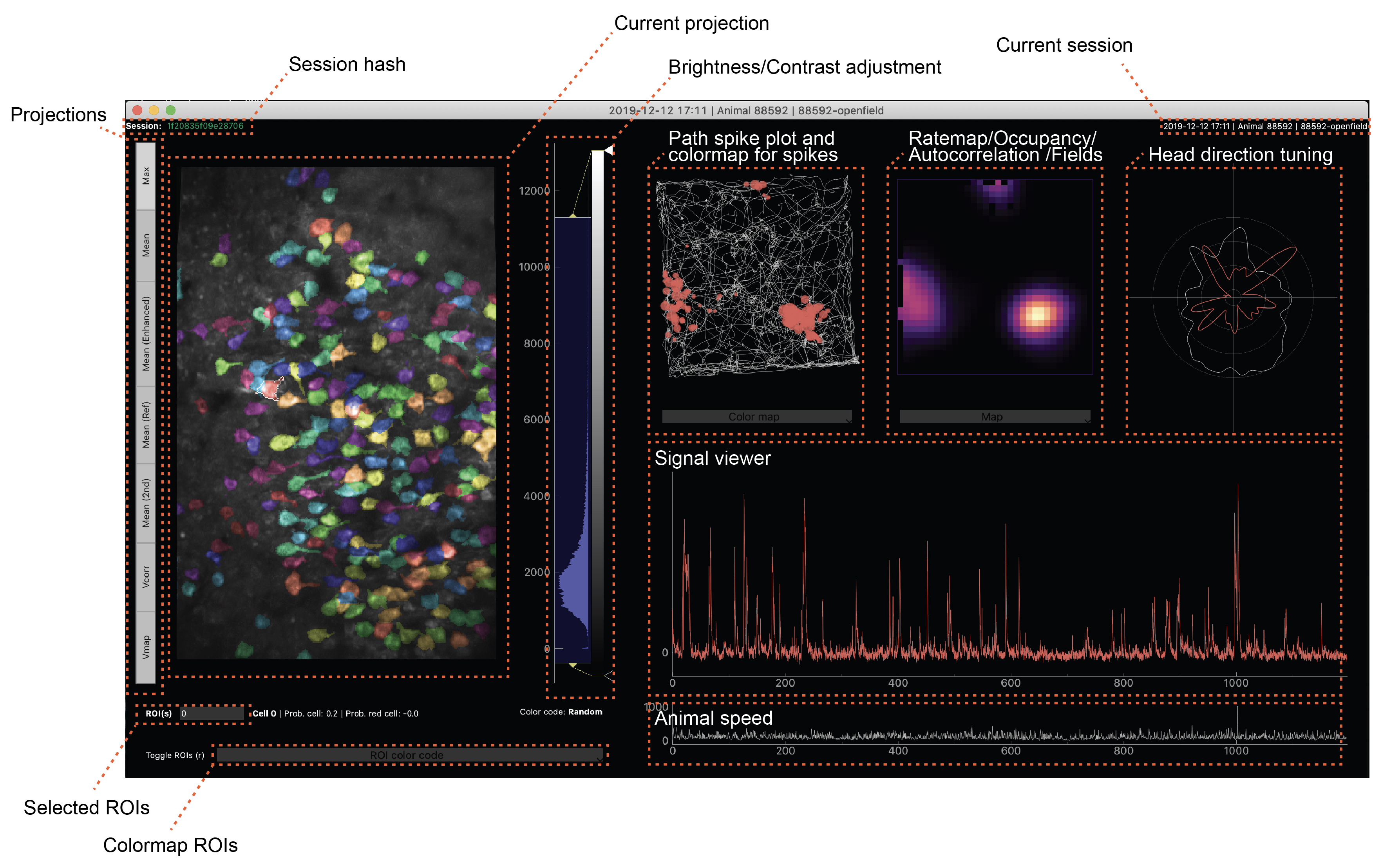
The main window is separated into a projection view (left), analysis views for experiments run in 2D environments (top right), a signal viewer (middle right), and a speed plot (bottom right). The GUI is able to display head fixed recordings as well (then the top right plots will stay black).

Upon loading a new session, projections/tracking/occupancy will be loaded from the database. Whenever the user clicks on a ROI on the left, the results for this ROI will be displayed on the right. Most plots allow zooming via the mouse wheel.

Keyboard shortcuts

Projection viewer

• R Show/hide ROIs. This will hide the color overlay of all ROIs and only show white outlines of selected ROIs.

• N Show/hide ROI numbers in projection view

Signal viewer

• S Show/hide deconvolved events

• D Show/hide fluorescent trace(s)

Plane selection (for multiplane imaging only)

• Q Plane up

• A Plane down

Parameter selection

• P Opens parameter selection window

Multiple ROIs

Multiple ROIs can be selected by either pressing down the shift key while clicking on ROIs or by typing out a comma separated list of valid ROI numbers into the field next to ROI(s) underneath the projection viewer and pressing enter. When multiple ROIs are selected, the results will be plotted together in the plots on the top right. Exceptions to this are the 2D occupancy view and field maps, which only shows the result of the last selected ROI.

What is displayed

Projection views

All results saved under Projection or ProjectionCorr in the imaging pipeline. ROI positions/pixels are loaded from Cell.Rois or RoisCorr. Whether corrected results are loaded or raw (/uncorrected) results only depends on whether a corrected result is available. Outlines and colormaps are calculated on the flow by retrieving results from matching tables in the database. The numbers match the cell_id attribute in the imaging pipeline.

Colormaps:

• Random: Random colors that are also used for events in the path events view, head direction tuning plot, and for signal and events in the signal viewer on the right.

• SNR: Signal to noise ratio (deltaF/F trace), loaded from SNR

• Spatial info content: Spatial information content loaded from Ratemap.Stats

• Gridscore: Loaded from GridScore

• MVL: Mean vector length (head direction tuning), loaded from AngularRate.Stats

• Borderscore: Loaded from BorderScore

The brightness and contrast of this figure can be adjusted by modifying the histogram handles displayed next to the projection viewer (see “Brightness/Contrast adjustment” in figure above). The brightness/contrast of every projection view can be individually adjusted.

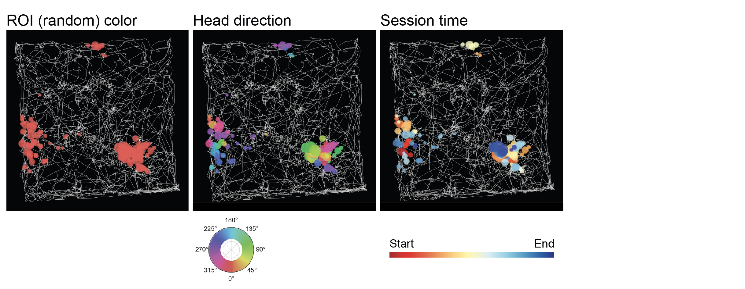
Path event plot

Displays the path retrieved from Tracking and deconvolved events from FilteredEvents. The event dot size corresponds to their amplitude. By clicking on the drop down menu underneath, several colormaps can be chosen:

Tuning map / … plots

Displays the 2D spatial tuning map by default (retrieved from TuningMap). By clicking on the drop down menu underneath, several other maps can be chosen:

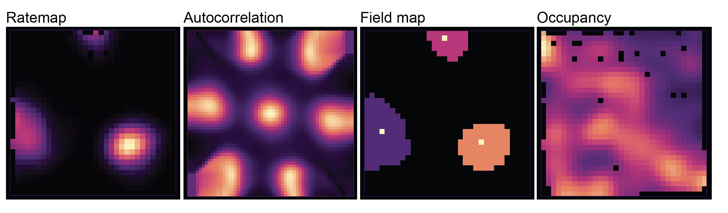
• Autocorrelation: 2D autocorr (acorr) from GridScore.

• Field map: All fields extracted from current tuning map, retrieved from TuningMap.Fields. Bright dots indicate field centroids (attribute field_centroid_x/field_centroid_y), which are overlaid after drawing the fields themselves.

• Occupancy: 2D occupancy retrieved from Occupancy.

Head direction tuning

Results are retrieved from AngularOccupancy (occupancy in white) and AngularTuning.

Signal viewer

Neuropil corrected traces from Cell.Traces (attribute fcorr, channel primary) and deconvolved events from FilteredEvents.

Subject speed

This is the speed attribute retrieved either from Tracking.OpenField (for 2D tracked sessions) or Tracking.Linear() for head fixed (1D) sessions.

Parameter selection

By typing P, a parameter selection window can be opened. This displays parameter sets throughout the Imaging pipeline that results for this recording depend on. Selecting a different parameter set will auto-reload results and refresh their views in the main window. Only parameter sets that are available (= have results calculated) for this recording are shown. By clicking the triangle displayed next to each parameter set, an overview of the different parameter sets and each parameter can be shown.

Save figures

Some plots allow right clicks to display context menus. These menus allow export of the selected plots (both as pixel as well as vector graphics).