Common Pipeline Conventions

Language

The pipeline code is written in a mixture of Python and Matlab.

Documentation is written in English. Where there exist differences in dialects of English, American English is standard, e.g., “color” instead of “colour”.

The pipeline code and database accept text in the Danish unicode format. This supports the standard Latin alphabet, and the Norwegian/Danish characters æ ø å, as well as the Swedish variations. Support of other accented Latin characters (e.g. â or ü) have not been tested. No support is provided for non-Latin characters (e.g. Greek, Cyrillic, etc).

Date formats

Date formats are generally given in ISO8601 format, i.e. YYYY-MM-DD. For example, November 9 1989 is given as 1989-11-09. Timestamps are typically provided accurate to the second, with missing information automatically filled in as zero. For example, 1989-11-09 will be converted to 1989-11-09 00:00:00

Folders and paths

All recording workstations, and the majority of researcher office computers run Windows, and therefore examples are primarily given for Windows.

It is generally assumed that the main Moser network drive is mounted as drive N:\

The Imaging file server can be mounted as any path, but is typically assumed to be mounted as F:\ and G:\

Coordinates

The calculation library opexebo uses the convention that co-ordinates should be given as (x, y) pairs, and all published functions have been tested as such.

NumPy typically uses the convention (y, x) - be very sure of which you are using! There are good reasons for the difference, tied to the history of the language C, and its role as a general purpose programming language rather than a mathematical tool (as Matlab and its predecessor Fortran were).

Angles

User-facing angles are typically in degrees.

For ease of computation, angles in tables mostly used for intermediate calculation are in radians.

If you are in any doubt which is which, check the table description, or check the maximum value stored in that column. Any values exceeding 6.283 (2 pi) indicates that the angles are stored in degrees. The column description will also state the units (accessible via table.describe()).

Angles are referenced to the X axis, i.e:

• 0° (=0 rad) points from the origin (x=0,y=0) towards the point (x=1, y=0). i.e. along the X-axis in the positive direction

• 90° (=pi/2 rad) points from the origin (x=0, y=0) towards the point (x=0, y=1). i.e. along the Y-axis in the positive direction

Coordinates, images, and imshow

The function imshow, in both Matlab or in matplotlib in Python, is a common source of confusion when comparing spatial and angular data.

Conventionally, a graph is plotted with (x=0, y=0) at the bottom left, with y increasing towards the top of the page and x increasing towards the right hand side of the page.

However, images are conventionally plotted upside down - with (x=0, y=0) at the top left; y increasing towards the bottom of the page, and x still increasing towards the right hand side of the page.

This is most relevant when you are comparing images (e.g. a ratemap) with an angular plot, e.g. a head direction tuning curve. Intuitively, we consider an angle of 90° (=pi/2 rad) to point upwards, i.e. to (x=0, y=1). However, in the conventional image plotting approach, the unit vector (0, 1) points down, not up.

Consider the following simple example:

import numpy as np
import matplotlib.pyplot as plt

null_image = np.eye(4)  # Example image to plot
vector_x = (0, 3)       # Example vector data
vector_y = (0, 3)       # example vector data

fig, (ax0, ax1, ax2) = plt.subplots(nrows=1, ncols=3, subplot_kw={"aspect":"equal"})

ax0.imshow(null_image)
ax0.plot(vector_x, vector_y, "--")
ax0.set_title("Image plot")

ax1.plot(vector_x, vector_y, "--")
ax1.set_title("Graph plot")

ax2.imshow(null_image)
ax2.invert_yaxis()
ax2.plot(vector_x, vector_y, "--")
ax2.set_title("Reversed Image Plot")

plt.show()

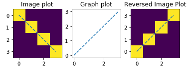
All three axes plot exactly the same (3, 3) vector. The first and final axes show exactly the same matrix (the identity matrix). The only distinction is the default way matplotlib chooses to display the y axis, and whether the user chooses to exert control over that choice of visualisation: in the first plot, y=0 is at top-left, and in the second and third plots, y=0 is at bottom-left.

Comparing open field and angular tracking

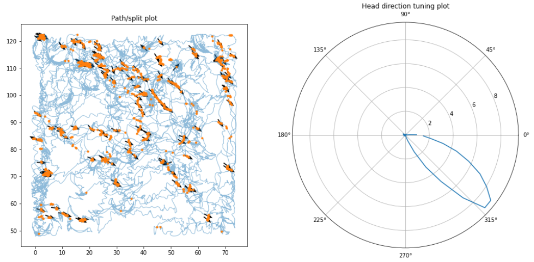
Due to the confusion introduced by the y-axis inversion of imshow, it can be quite confusing to be confident that your head-angle plots agree with your open field plots.

The easiest way to compare this is to directly plot head angles on a path/spike plot using Matplotlib’s quiver function (docs here)

The below code gives a specific example from the Ephys pipeline

key = {"animal_id":"8931a088caf410cf", "session_time":"2017-03-20 11:34:40", "unit":4016, "cluster_param_name":"default_klustakwik", "task_spike_tracking_hash":"90cf03aa63db1a03ac6dabe2cac2d108"}
trk = (analysis.TaskTracking & key).fetch1()
spk = (analysis.TaskSpikesTracking & key).fetch1()
hd = (analysis.HDTuning & key).fetch1()
hd_angles = (analysis.AngularOccupancy & key).fetch1("angle_centers")

# arrow_unit_vectors:
i = 10
angles_radians = spk["head_yaw"][::i]
u, v = np.cos(angles_radians), np.sin(angles_radians)

fig = plt.figure(figsize=(16,10))
ax = (fig.add_subplot(121), fig.add_subplot(122, projection="polar"))

ax[0].plot(trk["x_pos"], trk["y_pos"], alpha=0.5, linewidth=1)
ax[0].plot(spk["x_pos"], spk["y_pos"], ".")
ax[0].quiver(spk["x_pos"][::i], spk["y_pos"][::i], u, v, pivot="mid", linewidth=1, scale_units="width", headwidth=4, minshaft=2)
ax[0].set_aspect(1)
ax[0].set_title("Path/split plot")

ax[1].plot(hd_angles, hd["hd_tuning"])
ax[1].set_title("Head direction tuning plot")

Tracking and mirror-flips

Camera-based tracking in both the ephys and imaging pipelines raise some questions about co-ordinate conventions beyond those introduced by imshow.

The fundamental unit of tracking is the co-ordinate of a pixel within the camera. Different cameras may have different conventions about how this is labelled, which may introduce Up/Down and/or Left/Right flips compared to your expectations.

Hardware systems like Axona also include their own data visualisation, which may introduce their own data manipulation to compensate for the known behaviour of the attached camera. Data extraction into the pipelines does not take these unknown data manipulation into account. Data ingested into the pipelines uses the raw data format, whatever that format is without additional manipulation.

It is the responsibility of the user to identify what, if any, manipulation is required to match the actual data with their expectations (for example, to correctly identify where the cue card exists within the camera’s reference frame). Comparing the path plot to the tracking video is the best way to compare these two sets of data